Steve Bennett blogs

…about maps, open data, Git, and other tech.

Tag Archives: mapbox

Host your own vector tile server on Glitch

Most of the time, when you need to host vector tiles, you’ll use one of the two main (only?) commercial vector tile hosting services: Mapbox or Maptiler Cloud. But what if you don’t want to? Maybe you want to host tiles which don’t meet Mapbox’s 500KB-per-tile limit. Maybe you have some very specific requirement which can’t be met by those services.

We’ll use Glitch: your free NodeJS server edited through a web interface.

And Tessera: a NodeJS vector tile server. You tell it where your .mbtiles files are, and it serves them through an HTTP interface.

1. Create a project

We actually won’t use any of the provided template at all. You can start with the hello-express template.

Screen Shot 2019-12-18 at 11.23.50 am

2. Install Tessera

The easiest way to add dependencies is to select “package.json” then click “Add Package”.

  1. Add “tessera”.
  2. Add “mbtiles”. (By default Tessera doesn’t actually support mbtiles files. It’s a bit weird.)

Actually, because of a weird disagreement between Tessera and Glitch about the interpretation of a non-standard obscure HTTP header, you’ll have to use my patched version instead. Add this dependency directly into the package.json:

“tessera”: “stevage/tessera.git#x-forwarded-proto”

Now, we need to tell Glitch to run Tessera instead of the templated code that was set up for us. Change the “scripts” section to look like this:

Screen Shot 2019-12-18 at 10.05.29 am

3. Upload your .mbtiles file

Under “New File”, select “Upload a file”. Pick an .mbtiles file you have, upload and wait.

Screen Shot 2019-12-18 at 9.52.49 am

4. Really upload your .mbtiles file

Now, here’s the one tricky, rather clunky step. The asset you uploaded will actually live on Glitch’s assets CDN. It needs to be inside your server, so that Tessera can access it.

Inside the Glitch console (under “Tools”), first find out where the mbtiles file is, by running “less .glitch-assets”.

Look for a line like:

{“name”:”lgas.mbtiles”,”date”:”2019-12-17T22:56:15.660Z”,”url”:”https://cdn.glitch.com/982234c74-247f-4e51-9416-944436678291%2Flgas.mbtiles”

Extract out that url, and download it, choosing a sensible name:

$ wget -O lgas.mbtiles “https://cdn.glitch.com/982234c74-247f-4e51-9416-944436678291%2Flgas.mbtiles”

5. Configure Tessera

Now we’re going to make the config.json file promised in our package.json. In the main editor, create a new file, config.json.

My tiles contain local government areas (lgas), so this is what my config.json looks like:

Screen Shot 2019-12-18 at 10.12.18 am

Make sure the URL there points to the location of your specific file. It must start with “mbtiles://./”.

6. Test

Under “Show”, choose “Next to the Code” so we can whether Tessera is running correctly.

Click “Change URL” to access the TileJSON for your tile layer. In my case that looks like:

Screen Shot 2019-12-18 at 10.15.29 am

Check the JSON carefully. If you see ”

"filesize":0

or

"format":"png"

it means that Tessera couldn’t find your .mbtiles file, and created a blank one, assuming the file format was .png. (Yes, these are some interesting choices.)

7. Use your tiles!

You can now use your tiles in any Mapbox-GL-JS project. Instead of an identifier like “mapbox://stevage.nt2h43nh”, you’ll have a URL like “https://demo-tessera.glitch.me/lgas/index.json”. (You can use either HTTP or HTTPS – Glitch and Tessera support both.)

For instance, using mapbox-gl-utils:

Screen Shot 2019-12-18 at 11.21.35 am

Screen Shot 2019-12-18 at 11.17.08 am

You might not need PostGIS: streamlined vector tile processing for big map visualisations

I recently re-engineered the data processing behind OpenTrees.org. It’s a website that lets you explore the combined open tree databases of 21 local councils around Australia (over 800,000!), with some pretty data visualisations. Working on this site has taught me a lot about processing data into vector tiles. Today’s lesson: “You might not need PostGIS”.

Screenshot 2018-05-15 11.19.19.png

Trees from Melbourne, Hobson’s Bay and Brimbank.

First version: Tilemill, PostGIS, PGRestAPI

The architecture of v1 looked like this: (See “OpenTrees.org: how to aggregate 373,000 trees from 9 open data sources“).

  • Configuration file in JSON stores the location of each source file.
  • Bash scripts using JQ (yes, really) to run wget, ogr2ogr and psql to fetch, convert and load each datafile into PostGIS.
  • SQL scripts to merge and clean the datasets together into a single schema.
  • Tilemill to generate raster tiles from the data.
  • PGRestAPI to provide a queryable interface to the data (particularly to allow the map to zoom to a particular tree by ID).
  • Nginx serving the front end, built with Mapbox.js (a wrapper around Leaflet).
  • The magic of UTFGrid allows interrogating individual tree points. (I still love this technology.)

It worked fairly well, but with the huge disadvantage of having to host a web-accessible server, complete with database.

Second version: Mapbox-GL-JS, vector tiles, static hosting

When I lost access to my free hosting, I re-architected it using Mapbox-GL-JS: v2.

  • Same scripts to fetch and process data into PostGIS.
  • More scripts which export data out of PostGIS and call Tippecanoe to generate vector tiles, which I then upload to Mapbox.com.
  • No Tilemill
  • Brand new front-end built using Mapbox-GL-JS, with some clever new data visualisation, such as visualising by “rarity”.
  • No PGRestAPI. Clicking on a tree updates the URL to include its lat/long, so you have a shareable link that will go to that tree.
  • Front end hosted on Github Pages.

Now we don’t need a server (Github Pages and Mapbox are serving everything we need, and are free). But we still have the heavy dependency of PostGIS.

Do we really need PostGIS?

What is PostGIS actually doing in this scenario? Mostly it’s doing very simple row-oriented, non-relational operations like:

Screenshot 2018-05-15 10.35.52.png

or:

Screenshot 2018-05-15 10.36.24.png

(Yes, I should have used SPLIT_PART())

And then finally we just dump the whole table out to disk.

I began trying to replace it with Spatialite, but that didn’t seem to play very nicely with NodeJS for me. As soon as it got fiddly, the benefits of using it over Postgres began to disappear.

And why did I even need it? Mostly because I already had scripts in SQL and just didn’t want to rewrite them.

So, the disadvantages of PostGIS here:

  • It’s a big, heavy dependency which discourages any other contributors.
  • The data processing scripts have to be in SQL, which introduces a second language (alongside Javascript).
  • No easy way to generate newline-delimited GeoJSON (which would make generating vector tiles a bit faster.)

Third version: NodeJS, Mapbox

So, I rewrote it as v3:

  • Replaced the Bash scripts with NodeJS. Which means, instead of the nonsense of JQ, we have sensible looking Javascript for which the JSON config files work well.
  • Instead of loading Shapefiles into PostGIS, I convert everything into GeoJSON.
  • Instead of SQL “merge” scripts, a NodeJS script processes each tree then writes them all out as a single, line-delimited GeoJSON file.
  • Tippecanoe then operates on that file to generate vector tiles, which I upload to Mapbox.
  • Split the repository in two: one for the data processing (“opentrees-data“), and a separate one for the front end (“opentrees“). This seems to be a good pattern.

The workflow now looks like:

  1. 1-gettrees.js uses a configuration file to fetch datasets from predefined locations and save them, in whatever formats, in a standard place.
  2. 2-loadtrees.js converts each of these files into a geojson file using OGR2OGR.
  3. 3-processFiles.js loads each of these, processing all the individual trees into a standard schema, then writes out a single combined line-delimited GeoJSON.
  4. 4-vectorTiles.sh uses Tippecanoe to generate an mbtiles from the GeoJSON.

The processing scripts now look like:

Screenshot 2018-05-15 10.06.04.png

Screenshot 2018-05-15 10.07.11

For now, each GeoJSON file is loaded entirely in one synchronous load operation.

Screenshot 2018-05-15 10.41.32

(Processing all the GeoJSONs this way takes about 55 seconds on my machine. Loading them asynchronously reduces that to about 45. Most of the time is probably in the regular expressions.)

The only slight hurdle is generating the species count table. With PostGIS, this is just one more query run after all the others:

Screenshot 2018-05-15 10.23.15.png

In NodeJS, our “process each tree once” workflow can’t support this. After processing them once (counting species as we go), we process them all again to attach the species count attribute.

Screenshot 2018-05-15 10.19.27

If we were doing a lot of statistics, possibly PostGIS would start to look attractive again.

Do we really need OGR2OGR?

The next dependency I would like to remove is OGR2OGR. It is there because datasets arrive in formats I can’t control (primarily CSV, Shapefile, GeoJSON). I love using Mike Bostock’s shapefile library, but it doesn’t currently support projections other than EPSG:4326. That’s not a showstopper, just more work.

It would also be great not to have to maintain VRT files (in XML!) to describe the CSV formats in which data arrives.


OpenStreetMap vector tiles: mixing and matching engines, schemas and styles

For my next web mapping project, we’ll use vector tiles. Great. And the data will come from OpenStreetMap. Excellent. Now you only have five more questions to answer.

For the front-end web application developer who wants to stick a map in their site, vector tiles open up lots of options and flexibility, but also lots of choices.

  • Display engine: which JavaScript library is going to actually draw stuff in the browser?
  • Style: how will you tell the display engine what colour to draw each thing in the schema?
  • Data schema: what kinds of data are contained in the tiles, what are the layers called, and what are the attributes available?
  • Tile transport: how will the engine know where to get each tile from?
  • File format: how is the data translated into bytes to store within a tile file?

We’re very lucky that in a couple of these areas, a single standard dominates:

Which leaves three decisions to make.

Display engine

There are several viable options for displaying your vector tiles, depending on whether you also want to display raster tiles or need creative styling, if WebGL (IE11+ only) is ok, and what else you need to integrate with.

Screenshot 2017-08-22 23.26.11.png

Mapbox Terrain, a style rendered with Mapbox-GL-JS.

  • Mapbox-GL-JS: the industry leader, made by Mapbox, uses webGL, focused on the needs of mass-market maps for large web companies. It has excellent documentation, great examples and very active development.
  • Tangram: made by Mapzen, also uses WebGL, has more experimental and creative features like custom shaders.
  • OpenLayers: a fully-featured, truly open source mapping library primarily built for raster tiles, but with vector tile support. (Disclaimer: I’ve never used OpenLayers, I’m just reading docs here.)

There are other combinations as well, such as Leaflet.VectorGrid.

Style

The style mechanism tends to be closely tied to the display engine. (That was also true of CartoCSS, which was a pre-processor for Mapnik. RIP).

  • Mapbox Style Specification is a single JSON file which defines sources (vector tiles, GeoJSON files, raster tiles etc) and their display as layers (circles, fills, lines, text, icons etc), including properties that depend on zoom and/or data values. It also has some fiddly details for displaying custom fonts and symbols. Supported by Mapbox-GL-JS and Mapbox.js, but no third-party front-end libraries that I’m aware of. (Geoserver, a Java-based web application seems to have support.) Styles can be created with Mapbox Studio, Maputnik (free, open source) or by hand.
  • OpenLayers style is a JSON object for OpenLayers. It doesn’t seem to exist as a file format per se. (I’m not sure why the demo above just uses a ton of JavaScript statements rather than this style object.)
  • Tangram scene file, a YAML format which covers a bit more than just styling data, such as cameras and lighting.

Schema

Finally, there are three distinct, well-defined schemas for packaging OpenStreetMap data into vector tiles. There doesn’t seem to be a formal specification for how you define a schema, so each is presented as documentation: a list of layers, each with a list of attributes (and their possible values), and at which zoom levels they appear.

  • Mapbox Streets v7 (22 layers): a highly processed version of OpenStreetMap data optimised for simplicity and performance, geared towards general mapping applications. Layer and attribute names often reflect original OSM tag names (“waterway, class=stream”) but not slavishly (“road, class=link”, “road,
    Dark Matter (OpenMapTiles)

    Dark Matter, a Mapbox Style for OpenMapTiles.

    class=major_rail”).

  • OpenMapTiles (15 layers): an open schema developed by Klokan (a Swiss company) “in cooperation with the Wikimedia foundation”. It is a bit looser with layer names (“transportation, class=minor”) and occasionally quirky (“transportation, brunnel=tunnel”)
  • Mapzen (9 layers): includes both simplified “kind=” and original OSM “kind_detail=” tags on almost every object,  making them heavier than the alternatives. Somewhat confusingly, all waterway/water features are combined into a single layer and distinguished only by geometry (line or polygon). At lower zooms, data is sourced from Natural Earth, instead of OSM – I don’t know why. (A lot of work goes into these decisions!)

Matching schemas and styles

Now, the style needs to be designed for the schema: if the schema contains a layer called “roads”, your style can’t be expecting a layer called “transportation”. But it also needs to be expressed in the right format supported by the engine: don’t go feeding no YAML to Mapbox-GL-JS.

For instance:

  • Mapbox Basic uses the Mapbox Streets schema, and is expressed in the Mapbox
    Tron.png

    Tron, a highly stylised style from Mapzen for Tangram.

    Style Specification. And hence can be rendered by Mapbox-GL-JS, or OpenLayers. (Other standard Mapbox styles include Mapbox Streets, Mapbox Terrain and Mapbox Dark)

  • Cinnabar uses the Mapzen schema, and is expressed as a Tangram scene file. (Other Mapzen styles include Bubble Wrap, Tron, Zinc, Walkabout and Refill).
  • Klokantech Basic uses the OpenMapTiles schema, and is expressed in Mapbox-GL-JS. (Other OpenMapTiles styles include Positron, Dark Matter, OSM Bright, Toner and Fjord Color).

These styles kind of live within their company affiliations, however. How about styles rendered by one company’s engine, using data from a different schema:

  • Tilezen uses Mapzen’s schema, but is rendered with Mapbox-GL-JS. Demo. (There are also Mapzen examples for OpenLayers and D3). This token effort by Mapbox achieves the same thing.
  • This example uses OpenMapTiles, rendered using Tangram.

Mixing and matching

Which brings us to the point of this post. How do you mix schemas and styles? That is, how do you take a style you designed for Mapbox Streets, and make it work on OpenMapTiles? Or port one of Mapzen’s kooky open-licensed styles so it works with Mapbox Streets? Well, you can’t – yet.

(Adapting a style from one engine to another, like what ol-mapbox-style does, is a tough ask, because engines’ capabilities differ.)

But adapting a Mapbox Style file from one OpenStreetMap schema to another? That seems totally doable – even if there isn’t yet a tool to make that happen.

My quick little proof of concept in NodeJS converted OpenMapTiles’ “OSM Bright” style (left) to versions for Mapbox Streets (centre) and Mapzen (right).

Screenshot 2017-08-17 21.52.54

Want to give me a hand? Get in touch!


OpenTrees.org: how to aggregate 373,000 trees from 9 open data sources

I try to convince government bodies, especially local councils, to publish more open data. It’s much easier when there is a concrete benefit to point to: if you publish your tree inventory, it could be joined up with all the other councils’ tree inventories, to make some kind of big tree-explorey interface thing.

Introducing: opentrees.org. It’s fun! Click on “interesting trees”, hover over a few, and click on the ones that take your fancy. You can play for ages.

Here’s how I made it.

First you get the data

Through a bit of searching on data.gov.au, I found tree inventories (normally called “Geelong street trees” or similar) for: Geelong, Ballarat (both participating in OpenCouncilData), Corangamite (I visited last year), Colac-Otways (friends of Corangamite), Wyndham (a surprise!), Manningham (total surprise). It showed two results from data.sa.gov.au: Adelaide, and the Waite Arboretum (in Adelaide). Plus the City of Melbourne’s (open data pioneers) “Urban Forest” dataset on data.melbourne.vic.gov.au.

Every dataset is different. For instance:

  • GeoJSON’s for Corangamite, Colac-Otways, Ballarat, Manningham
  • CSV for Melbourne and Adelaide. Socrata has a “JSON” export, but it’s not GeoJSON.
  • Wyndham has a GeoJSON, but for some reason the data is represented as “MultiPoint”, rather than “Point”, which GDAL couldn’t handle. They also have a CSV, which are also very weird, with an embedded WKT geometry (also MULTIPOINT), in a projected (probably UTM) format. There are also several blank columns.
  • Waite Arboretum’s data is in zipped Shapefile and KML. KML is the worst, because it seems to have attributes encoded as HTML, so I used the Shapefile.

Source code for gettrees.sh.

Tip for data providers #1: Choose CSV files for all point data, with columns “lat” and “lon”. (They’re much easier to manipulate than other formats, it’s easy to strip fields you don’t need, and they’re useful for doing non-spatial things with.)

Then you load the data

Next we load all the data files, as they are, into separate tables in PostGIS. GDAL is the magic tool here. Its conversion tool, ogr2ogr, has a slightly weird command line but works very well. A few tips:

  • Set the target table geometry type to be “GEOMETRY”, rather than letting it choose a more specific type like POINT or MULTIPOINT. This makes it easier to combine layers later.
    -nlt GEOMETRY
  • Re-project all geometry to Web Mercator (EPSG:3857) when you load. Save yourself pain.
    -t_srs EPSG:3857
  • Load data faster by using Postgres “copy” mode:
    –config PG_USE_COPY YES
  • Specify your own table name:
    -nln adelaide

Tip for data providers #2: Provide all data in unprojected (latitude/longitude) coordinates by preference, or Web Mercator (EPSG:3857).

CSV files unfortunately require creating a companion ‘.vrt’ file for non-trivial cases (eg, weird projections, weird column names). For example:
<OGRVRTDataSource>
<OGRVRTLayer name="melbourne">
<SrcDataSource>melbourne.csv</SrcDataSource>
<GeometryType>wkbPoint</GeometryType>
<LayerSRS>WGS84</LayerSRS>
<GeometryField encoding="PointFromColumns" x="Longitude" y="Latitude"/>
</OGRVRTLayer>
</OGRVRTDataSource>

The command to load a dataset looks like:
ogr2ogr --config PG_USE_COPY YES -overwrite -f "PostgreSQL" PG:"dbname=trees" -t_srs EPSG:3857 melbourne.vrt -nln melbourne -lco GEOMETRY_NAME=the_geom -lco FID=gid -nlt GEOMETRY
Source code for loadtrees-db.sh.

Merge the data

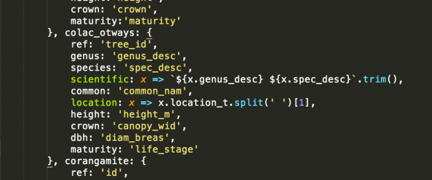
Unfortunately most councils do not yet publish data in the (very easy to follow!) opencouncildata.org standards. So we have to investigate the data and try to match the fields into the scheme. Basically, it’s a bunch of hand-crafted SQL INSERT statements like:
INSERT INTO alltrees (the_geom, ref, genus, species, scientific, common, location, height, crown, dbh, planted, maturity, source)
SELECT the_geom,
tree_id AS ref,
genus_desc AS genus,
spec_desc AS species,
trim(concat(genus_desc, ' ', spec_desc)) AS scientific,
common_nam AS common,
split_part(location_t, ' ', 1) AS location,
height_m AS height,
canopy_wid AS crown,
diam_breas AS dbh,
CASE WHEN length(year_plant::varchar) = 4 THEN to_date(year_plant::varchar, 'YYYY') END AS planted,
life_stage AS maturity,
'colac_otways' AS source
FROM colac_otways;

Notice that we have to convert the year (“year_plant”) into an actual date. I haven’t yet fully handled complicated fields like health, structure, height and dbh, so there’s a mish-mash of non-numeric values, different units (Adelaide records the circumference of trees rather than diameter!)

Tip for data providers #3: Follow the opencouncildata.org standards, and participate in the process.

Source code for mergetrees.sql

Clean the data

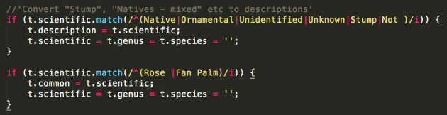
We now have 370,000 trees but it’s of very variable quality. For instance, in some datasets, values like “Stump”, “Unknown” or “Fan Palm” appear in the “scientific name” column. We need to clean them out:
UPDATE alltrees
SET scientific='', genus='', species='', description=scientific
WHERE scientific='Vacant Planting'
OR scientific ILIKE 'Native%'
OR scientific ILIKE 'Ornamental%'
OR scientific ILIKE 'Rose %'
OR scientific ILIKE 'Fan Palm%'
OR scientific ILIKE 'Unidentified%'
OR scientific ILIKE 'Unknown%'
OR scientific ILIKE 'Stump';

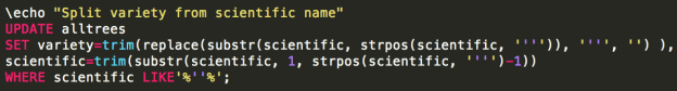
We also want to split scientific names into individual genus and species fields, handle varieties, sub-species and so on. Then there are the typos which, due to some quirk in tree management software, become faithfully and consistently retained across a whole dataset. This results in hundreds of Angpohoras, Qurecuses, Botlebrushes etc. We also need to turn non-values (“Not assessed”, “Unknown”, “Unidentified”) into actual NULL values.
UPDATE alltrees
SET crown=NULL
WHERE crown ILIKE 'Not Assessed';

Source code for cleantrees.sql

Tip for data providers #4: The cleaner your data, the more interesting things people can do with it. (But we’d rather see dirty data than nothing.)
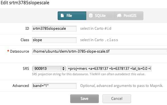
Make a map

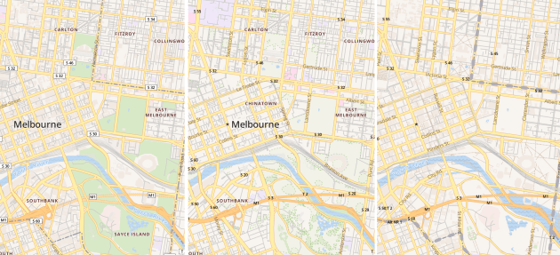
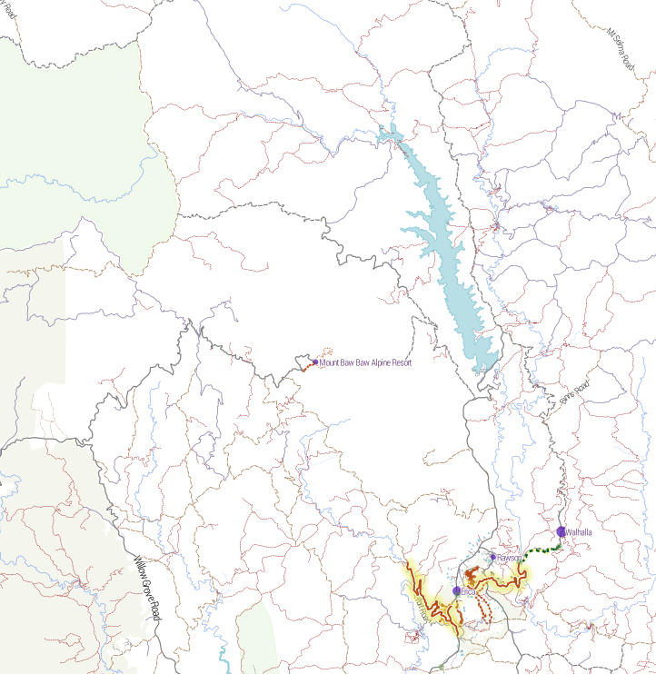
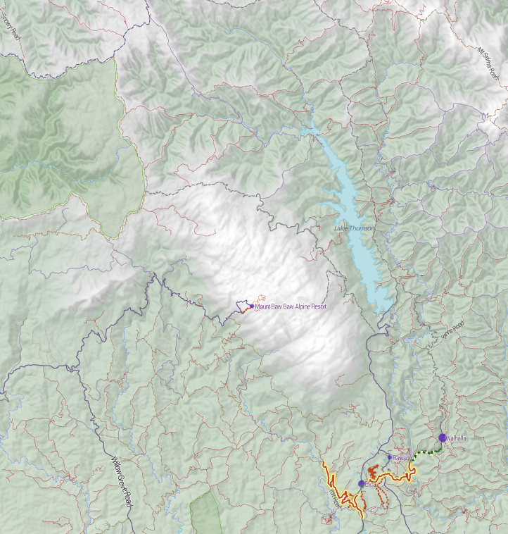
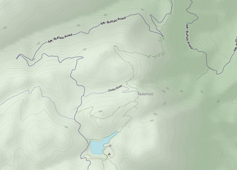
I use TileMill to make web maps. For this project it has a killer feature: the ability to pre-render a map of hundreds of thousands of points, and allow the user to interact with those points, without exploding the browser. That’s incredibly clever. Having complete control of the cartography is also great, and looks much better than, say, dumping a bunch of points on a Google Map.

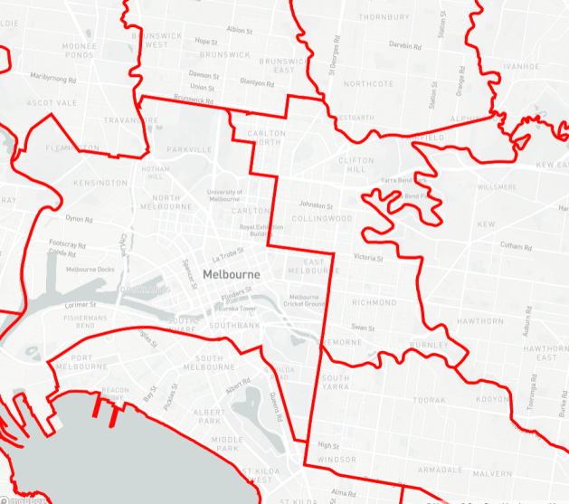
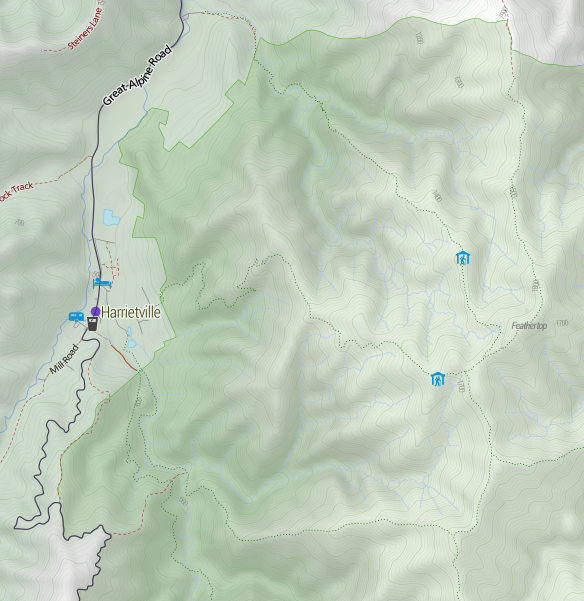
As far as TileMill maps goes, it’s very conventional. I add a PostGIS layer for the tree points, plus layers for other features such as roads, rivers and parks, pointing to an OpenStreetMap database I already had loaded. Also show the names of the local government areas with their boundaries, which fade out and disappear as you zoom in.

My style is intentionally all about the trees. There are some very discreet roads and footpaths to serve as landmarks, but they’re very subdued. I use colour (from green to grey) to indicate when species and/or genus information is missing. The Waite Arboretum data has polygons for (I presume) crown coverage, which I show as a semi-opaque dark green.

OpenTrees.org TileMill screenshot


Source code for the TileMill CartoCSS style.

There’s also an interactive layer, so the user can hover over a tree to see more information. It looks like this:
<b>{{{common}}} <i>{{{scientific}}}</i></b>
<br/>
<table>
{{#genus}}<tr><th>Genus </th><td>{{{genus}}}</td></tr>{{/genus}}
{{#species}}<tr><th>Species</th><td>{{{species}}}</td></tr>{{/species}}
{{#variety}}<tr><th>Variety</th><td>{{{variety}}}</td></tr>{{/variety}}

...
I also whipped up two more layers:

  1. OpenStreetMap trees, showing “natural=tree” objects in OpenStreetMap. The data is very sketchy. This kind of data is something that councils collect much better than OpenStreetMap.
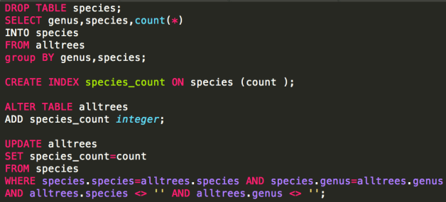
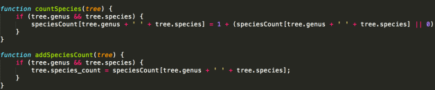
  2. Interesting trees. I compute the “interestingness” of a tree by calculating the number of other trees in the total database of the same species. A tree in a set of 5 or less is very interesting (red), 25 or less is somewhat interesting (yellow).

Source code for makespecies.sql.

Build a website

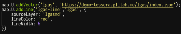
It’s very easy to display a tiled, interactive map in a browser, using Leaflet.JS and Mapbox’s extensions. It’s a lot more work to turn that into an interesting website. A couple of the main features:

  • The base CSS is Twitter Bootstrap, mostly because I don’t know any better.
  • Mapbox.js handles the interactivity, but I intercept clicks (map.gridLayer.on) to look up the species and genus on Wikipedia. It’s straightforward using JQuery but I found it fiddly due to unfamiliarity. The Wikipedia API is surprisingly rough, and doesn’t have a proper page of its own – there’s the MediaWiki API page, the Wikipedia API Sandbox, and this useful StackOverflow question which that community helpfully shut down as a service to humanity.
  • To make embedding the page in other sites (such as Open Council Data trees) work better, the “?embed” URL parameter hides the titlebar.
  • You can go straight to certain councils with bookmarks: opentrees.org/#adelaide
  • I found the fonts (the title font is “Lancelot“) on Adobe Edge.
  • The header background combines the forces of subtlepatterns.com and px64.net.

Source code for treesmap.html, treesmap.js, treesmap.css.

And of course there’s a server component as well. The lightweight tilelive_server, written mostly by Yuri Feldman, glues together the necessary server-side bits of MapBox’s technology. I pre-generate a large-ish chunk of map tiles, then the rest are computed on demand. This bit of nginx code makes that work (well, after tilelive_server generated 404s appropriately):
location /treetiles/ {
# Redirect to TileLive. If tile not found, redirect to TileMill.
rewrite_log on;
rewrite ^.*/(\d+)/(\d+)/(\d+.*)$ /supertrees_c8887d/$1/$2/$3 break;

proxy_intercept_errors on;
error_page 404 = @dynamictiles;
proxy_set_header Host $http_host;
proxy_pass http://127.0.0.1:5044;

proxy_cache my-cache;
}

location @dynamictiles {
rewrite_log on;
rewrite ^.*/(\d+)/(\d+)/(\d+.*)$ /tile/supertrees/$1/$2/$3 break;
proxy_pass http://guru.cycletour.org:20008;
proxy_cache my-cache;
}

Too hard basket

A really obvious feature would be to show native and introduced species in different colours. Try as I might, I could not find any database with this information. There are numerous online plant databases, but none seemed to have this information in a way I could access. If you have ideas, I’d love to hear from you.

It would also be great to make a great mobile app, so you can easily answer the question “what is this tree in front of me”, and who knows what else.

In conclusion

Dear councils,

  Please release datasets such as tree inventories, garbage collection locations and times, and customer service centres, following the open standards at opencouncildata.org. We’ll do our best to make fun, interesting and useful things with them.

Love,

The open data community

Terrain in TileMill: a walkthrough for non-GIS types

I created a basemap for http://cycletour.org with TileMill and OpenStreetMap. It looked…ok.

Image

But it felt like there was something missing. Terrain. Elevation. Hills. Mountains. I’d put all that in the too hard basket, until a quick google turned up two blog posts from MapBox, the wonderful people who make TileMill. “Working with terrain data” and “Using TileMill’s raster-colorizer“. Putting these two together, plus a little OCD, led me to this:

Image

Slight improvement! Now, I felt that the two blog posts skipped a couple of little steps, and were slightly confusing on the difference between the two approaches, so here’s my step by step. (MapBox, please feel free to reuse any of this content.)

My setup is an 8 core Ubuntu VM with 32GB RAM and lots of disk space. I have OpenStreetMap loaded into PostGIS.

1. Install the development version of TileMill

You need to do this if you want to use the raster-colorizer. You want this while developing your terrain style, if you want the “snow up high, green valleys below” look. Without it, you have to pre-render the elevation color effect, which is time consuming. If you want to tweak anything (say, to move the snow line slightly), you need to re-render all the tiles.

Fortunately, it’s pretty easy.

  1. Get the “install-tilemill” gist (my version works slightly better)
  2. Probably uncomment the mapnik-from-source line (and comment out the other one). I don’t know whether you need the latest mapnik.
  3. Run it. Oh – it will uninstall your existing TileMill. Watch out for that.
  4. Reassemble stuff. The dev version puts projects in ~/Documents/<username/MapBox/project which is weird.

2. Get some terrain data.

The easiest place is the ubiquitous NASA SRTM DEM (digital elevation model) data. You get it from CGIAR. The user interface is awful. You can only download pieces that are 5 degrees by 5 degrees, so Victoria is 4 pieces.

Screen shot 2013-09-11 at 10.46.00 PM

If you’re downloading more than about that many, you’ll probably want to automate the process. I wrote this quick script to get all the bits for Australia:

for x in {59..67}; do
for y in {14..21}; do
echo $x,$y
if [ ! -f srtm_${x}_${y}.zip ]; then
wget http://droppr.org/srtm/v4.1/6_5x5_TIFs/srtm_${x}_${y}.zip
else
echo "Already got it."
fi
done
done
unzip '*.zip'


3. Process SRTM .tifs with GDAL.

To have any fun with terrain mapping in TileMill, you need to produce separate layers from the terrain data:

  1. The heightmap itself, so you can colour high elevations differently from low ones.
  2. A “hillshading” layer, where southeast facing slopes are dark, and northwest ones are light. This is what produces the “terrain” illusion.
  3. A “slopeshading” layer, where steep slopes (regardless of aspect) are dark. I’m ambivalent about how useful this is, but you’ll want to play with it.
  4. Contours. These can make your map look AMAZING.
Screen shot 2013-09-11 at 10.53.41 PM

Contours – they’re the best.

In addition, you’ll need some extra processing:

  1. Merge all the .tif’s into one. (I made the mistake of keeping them separate, which makes a lot of extra layers in TileMill). Because they’re GeoTiffs, GDAL can magically merge them without further instruction.
  2. Re-project it (converting it from some random ESPG to Google Web Mercator – can you tell I’m not a real GIS person?)
  3. A bit of scaling here and there.
  4. Generating .tif “overviews”, which are basically smaller versions of the tifs stored inside the same file, so that TileMill doesn’t explode.

Hopefully you already have GDAL installed. It probably came with the development version of TileMill.

Here’s my script for doing all the processing:

#!/bin/bash
echo -n "Merging files: "
gdal_merge.py srtm_*.tif -o srtm.tif
f=srtm
echo -n "Re-projecting: "
gdalwarp -s_srs EPSG:4326 -t_srs EPSG:3785 -r bilinear $f.tif $f-3785.tif

echo -n "Generating hill shading: "
gdaldem hillshade -z 5 $f-3785.tif $f-3785-hs.tif
echo and overviews:

gdaladdo -r average $f-3785-hs.tif 2 4 8 16 32
echo -n "Generating slope files: "
gdaldem slope $f-3785.tif $f-3785-slope.tif
echo -n "Translating to 0-90..."
gdal_translate -ot Byte -scale 0 90 $f-3785-slope.tif $f-3785-slope-scale.tif
echo "and overviews."
gdaladdo -r average $f-3785-slope-scale.tif 2 4 8 16 32
echo -n Translating DEM...
gdal_translate -ot Byte -scale -10 2000 $f-3785.tif $f-3785-scale.tif
echo and overviews.
gdaladdo -r average $f-3785-scale.tif 2 4 8 16 32
#echo Creating contours
gdal_contour -a elev -i 20 $f-3785.tif $f-3785-contour.shp

Take my word for it that the above script does everything I promise. The options I’ve chosen are all pretty standard, except that:

  • I’m exaggerating the hillshading by a factor of 5 vertically (“-z 5”). For no particularly good reason.
  • Contours are generated at 20m intervals (“-i 20”).
  • Terrain is scaled in the range -10 to 2000m. Probably an even lower lower bound would be better (you’d be surprised how much terrain is below sea levels – especially coal mines.) Excessively low terrain results in holes that can’t be styled and turn up white.

4. Load terrain layers into TileMill

Now you have four useful files, so create layers for them. I’d suggest creating them as layers in this order (as seen in TileMill):

  1. srtm-3785-contour.shp – the shapefile containing all the contours.
  2. srtm-3785-hs.tif – the hillshading file.
  3. srtm-3785-slope-scale.tif – the scaled slope shading file.
  4. srtm-3785.tif – the height map itself. (I also generate srtm-3785-scale.tif. The latter is scaled to a 0-255 range, while the former is in metres. I find metres makes more sense.)

For each of these, you must set the projection to 900913 (that’s how you spell GOOGLE in numbers). For the three ‘tifs’, set band=1 in the “advanced” box. I gather that GeoTiffs can have multiple bands of data, and this is the band where TileMill expects to find numeric data to apply colour to.

Screen shot 2013-09-11 at 11.06.39 PM

5. Style the layers

Mapbox’s blog posts go into detail about how to do this, so I’ll just copy/paste my styles. The key lessons here are:

  • Very slight differences in opacity when stacking terrain layers make a huge impact on the appearance of your map. Changing the colour of a road doesn’t make that much difference, but with raster data, a slight change can affect every single pixel.
  • There are lots of different raster-comp-ops to try out, but ‘multiply’ is a good default. (Remember, order matters).
  • Carefully work out each individual zoom level. It seems to work best to have hillshading transition to contours around zoom 12-13. The SRTM data isn’t detailed enough to really allow hillshading above zoom 13

My styles:

.hs[zoom <= 15] {
[zoom>=15] { raster-opacity: 0.1; }
[zoom>=13] { raster-opacity: 0.125; }
[zoom=12] { raster-opacity:0.15;}
[zoom<=11] { raster-opacity: 0.12; }
[zoom<=8] { raster-opacity: 0.3; }

raster-scaling:bilinear;
raster-comp-op:multiply;
}

// not really convinced about the value of slope shading
.slope[zoom <= 14][zoom >= 10] {
raster-opacity:0.1;
[zoom=14] { raster-opacity:0.05; }
[zoom=13] { raster-opacity:0.05; }
raster-scaling:lanczos;
raster-colorizer-default-mode: linear;
raster-colorizer-default-color: transparent;

// this combo is ok
raster-colorizer-stops:
stop(0, white)
stop(5, white)
stop(80, black);
raster-comp-op:color-burn;

}

// colour-graded elevation model
.dem {
[zoom >= 10] { raster-opacity: 0.2; }
[zoom = 9] { raster-opacity: 0.225; }
[zoom = 8] { raster-opacity: 0.25; }
[zoom <= 7] { raster-opacity: 0.3; }
raster-scaling:bilinear;
raster-colorizer-default-mode: linear;
raster-colorizer-default-color: hsl(60,50%,80%);
// hay, forest, rocks, snow

// if using the srtm-3785-scale.tif file, these stops should be in the range 0-255.
raster-colorizer-stops:
stop(0,hsl(60,50%,80%))
stop(392,hsl(110,80%,20%))
stop(785,hsl(120,70%,20%))
stop(1100,hsl(100,0%,50%))
stop(1370,white);
}
.contour[zoom >=13] {
line-smooth:1.0;
line-width:0.75;
line-color:hsla(100,30%,50%,20%);
[zoom = 13] {
line-width:0.5;
line-color:hsla(100,30%,50%,15%);
}

[zoom >= 16],
[elev =~ “.*00”] {
l/text-face-name:’Roboto Condensed Light’;
l/text-size:8;
l/text-name:'[elev]’;
[elev =~ “.*00”] { line-color:hsla(100,30%,50%,40%); }
[zoom >= 16] { l/text-size: 10; }
l/text-fill:gray;
l/text-placement:line;
}
}

And finally a gratuitous shot of Mt Feathertop, showing the major approaches and the two huts: MUMC Hut to the north and Federation Hut further south. Terrain is awesome!

Screen shot 2013-09-11 at 11.25.23 PM